Research
Overview
I develop and analyze numerical methods that come with guarantees for evolution problems whose difficulty stems from two features that classical solvers handle poorly:
- Nonlocality — interactions over a finite or infinite range, as in fractional and tempered-stable (Lévy) operators and in nonlocal models of fracture; and
- Constraints — obstacles, free boundaries, irreversible damage, and contact.
These features govern the pricing of early-exercise and credit-risky contracts in finance and the fracture and crushing of brittle solids and granular media in mechanics — the two application areas that anchor my work. My research proceeds on three connected levels: analysis of the continuous models (well-posedness, energy balance, thermodynamic consistency), structure-preserving discretizations that retain the property responsible for stability (coercivity, inf-sup, cancellation, positivity) and are proved to converge, and certified computation — computable, rigorous error bounds that let one trust a computed, or machine-learned, answer. The question tying these together grows more pressing as scientific machine learning enters practice: when can we certify that a computed solution is correct?
My training spans both applied mathematics and computational engineering (two Ph.D.s, Mississippi State), and my postdoctoral work in Robert Lipton’s group at LSU — funded by two DoD MURI awards — lets me move between rigorous analysis, algorithm design, and large-scale simulation.
Constrained & free-boundary problems
Realistic contracts and physical processes are shaped by a constraint: early exercise, a barrier, path dependence, default, or irreversible contact. The constraint turns the governing equation into a variational inequality or a free-boundary problem, and that is where most of the financially and physically relevant information sits — the early-exercise boundary, the default threshold, the crack front.
Space–time least-squares methods for obstacle problems
With collaborators in Chile I co-developed a space–time finite element method for the parabolic obstacle problem \(\partial_t u + Lu \ge f,\; u \ge g,\; (\partial_t u + Lu - f)(u-g) = 0\) with a general convection–diffusion–reaction operator \(L\) — which includes Black–Scholes in log-price, so the American put is a special case. Introducing the flux \(\sigma = -A\nabla u\) and the reaction force (the early-exercise premium density) \(\lambda = \partial_t u + Lu - f\) turns the problem into a first-order system whose variational inequality has a symmetric, bounded, coercive bilinear form. We proved quasi-optimality (a Céa–Falk lemma) for any discrete convex set and a reliable a-posteriori estimator that drives simultaneous space–time adaptivity following the free boundary. For the American put, adaptivity restores the optimal rate \(O((\#\mathcal{P})^{-1/2})\), compared with \(O((\#\mathcal{P})^{-3/8})\) on uniform meshes. (Carvajal, Damircheli, Führer, Fuica, Karkulik, IMA J. Numer. Anal., 2025)
Minimum-residual (DPG) methods for option pricing
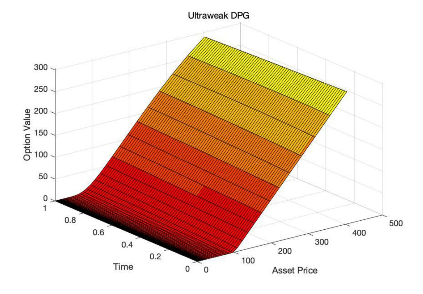
My doctoral work in computational engineering brought discontinuous Petrov–Galerkin (DPG) methods to option pricing, including American options solved by semismooth Newton methods on the symmetric positive-definite DPG system. I have since built a rigorous theory: for the correlated \(d\)-asset Black–Scholes operator I proved mesh-independent inf-sup stability for both the primal and the ultraweak formulations — the latter with no compatibility condition — and constructed a uniformly bounded Fortin operator that makes the practical method unconditionally stable and quasi-optimal. Because DPG minimizes the residual in a norm chosen for stability, it carries a built-in error estimator, and the Greeks (Delta, Gamma, cross-Gamma) are read directly from the first-order variables, with no numerical differentiation of prices. (preprint)
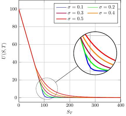
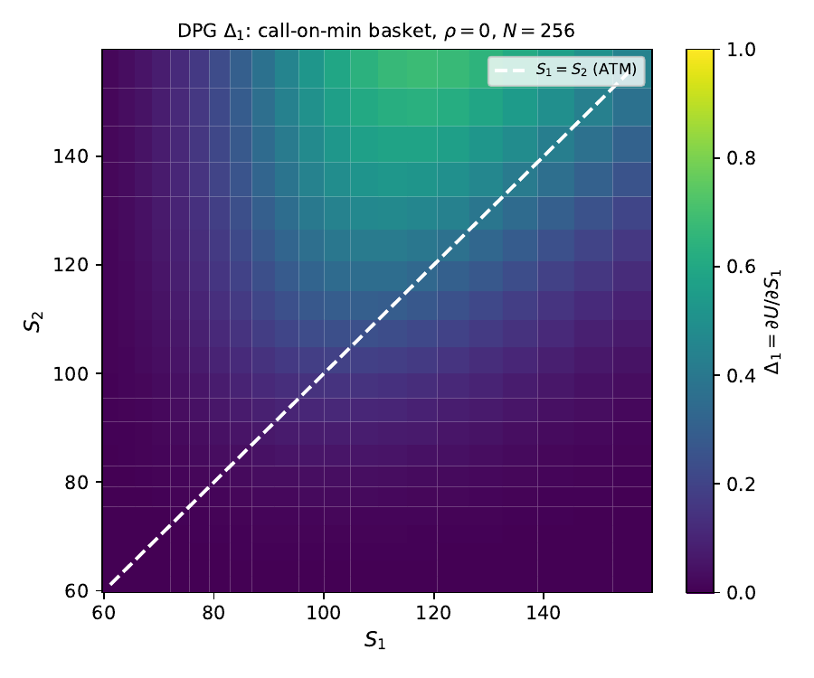
For degenerate and path-dependent contracts I identified the weighted space \(H^1_z = \{u : z\,u_z \in L^2\}\) appropriate to the interior-degenerate Asian operator, and showed that discrete barrier monitoring is an \(L^2\)-nonexpansive projection — a clean separation from the PDE step that leaves no value outside the knock-out corridor.
Free boundaries with solution-dependent coefficients
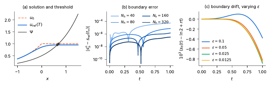
In the credit-rating migration model the volatility of a corporate bond switches when the firm crosses an unknown rating threshold, so the coefficients depend nonlocally on the solution itself. I introduced a recovered-coefficient discontinuous Galerkin method in which the coefficients are evaluated on a recovered state built from local averaging, the model’s own mollifier, and a computable cutoff. The recovery map is Lipschitz into \(W^{2,\infty}\) uniformly in \(h\), has the exact solution as a fixed point, and switches off for small \(h\) and \(\Delta t\). This yields an \(O(h^p + \Delta t)\) energy estimate, an error bound for the location of the migration boundary, and a clean separation between discretization and modeling errors. (preprint, arXiv:2107.09248)
Structure-preserving methods for nonlocal operators
Fractional and Lévy operators produce dense, singular, nonlocal matrices — the reason they are expensive and why naive surrogates struggle. I design discretizations that keep their hidden structure (Toeplitz, coercivity, exact cancellation), so the discrete method inherits the continuous stability constants.
Exact Galerkin assembly for the fractional Laplacian
Assembling the integral fractional Laplacian \((-\Delta)^s\) is the bottleneck of nonlocal finite elements. With M. Razzaghi and T. N. Vo I identified why closed-form assembly from pointwise cell actions fails for \(s \ge \tfrac12\): a discontinuous cell polynomial generates a non-integrable endpoint singularity. Imposing the shared nodal value before termwise integration produces a second-order algebraic cancellation, after which every interaction class (coincident, touching, separated) has a finite closed form for all \(0 < s < 1\). Using a one-dimensional Faermann-type localization of the Gagliardo seminorm, we proved optimal convergence on graded meshes for every \(0 < s < 1\) under a grading condition much weaker than the one from global interpolation. A multidimensional version based on Lauricella-type hypergeometric functions is in progress.
Tempered-stable (CGMY / Lévy) dynamics and calibration to data
Under the CGMY process the pricing operator contains tempered fractional derivatives of order \(Y \in (0,2)\) — dense, singular, and nonlocal. I derived exact Fourier-symbol connection coefficients for the exponentially conjugated tempered Riemann–Liouville operators in a B-spline basis; the resulting matrices are exactly Toeplitz and applied by FFT in \(O(N \log N)\). A monotonicity lemma for the symbol gives \(\operatorname{Re}\mathcal{A}(\xi) \ge r\), hence coercivity whenever the interest rate is positive, and interior-supported splines make the discrete stiffness an exact Toeplitz section — so the continuous bounds are inherited with the same constants. I proved the fully discrete rate \(O(h^{p - Y/2} + \Delta\tau^2)\) for \(Y \in (1,2)\). (preprint, arXiv:2610.07554)
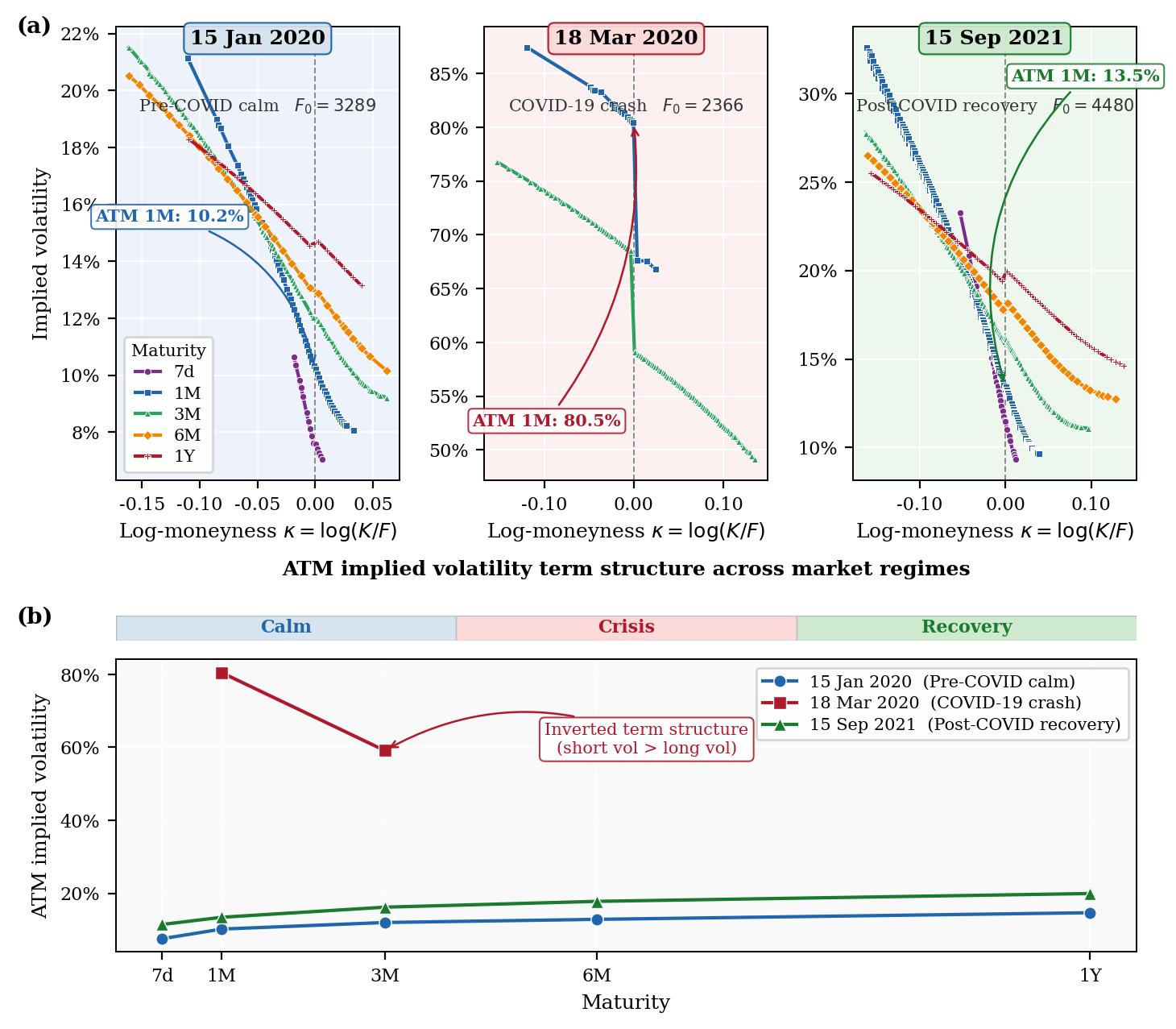
A pricing method is useful only if the model it solves can be fitted to the market. I calibrated the five CGMY parameters to S&P 500 option quotes across three market regimes — calm, crisis, and recovery — with the B-spline solver inside the optimization loop. The calibrated parameters carry economic information: the jump-activity parameter rises sharply in the crisis regime, a quantitative signature of market stress read directly from option prices.
In structural credit models with a Markov-modulated Lévy firm value and synchronous jumps at regime changes, default probabilities solve a coupled system of PIDEs with a singular jump integral. I proved that the compensated jump integral is finite for every generalized tempered-stable Lévy measure with activity below 2 — a family that covers variance gamma, CGMY, KoBoL, and bilateral gamma — so radial-basis collocation is de-singularized automatically, with no truncation of small jumps. (Damircheli, Razzaghi, Kazemi, Foroush Bastani, Eng. Anal. Bound. Elem., 2023) My earlier work developed radial-basis collocation for American options under regime-switching jump-diffusion models. (Foroush Bastani, Ahmadi, Damircheli, Appl. Numer. Math., 2013)
Anomalous (subdiffusive) and fractional dynamics
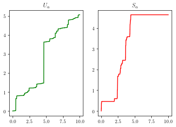
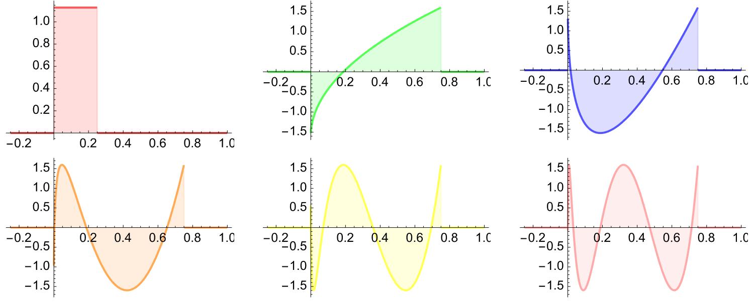
In illiquid markets prices can stay flat for random periods. Modeling the underlying as geometric Brownian motion time-changed by an inverse \(\alpha\)-stable subordinator leads to a time-fractional Black–Scholes equation. For it I developed fractional-order Taylor-/Chebyshev-wavelet collocation in which the Riemann–Liouville integrals of the basis are computed exactly through the regularized beta function, and the same exact-operator approach extends to other time–space fractional transport problems. (wavelet collocation, Numer. Methods PDEs, 2024)
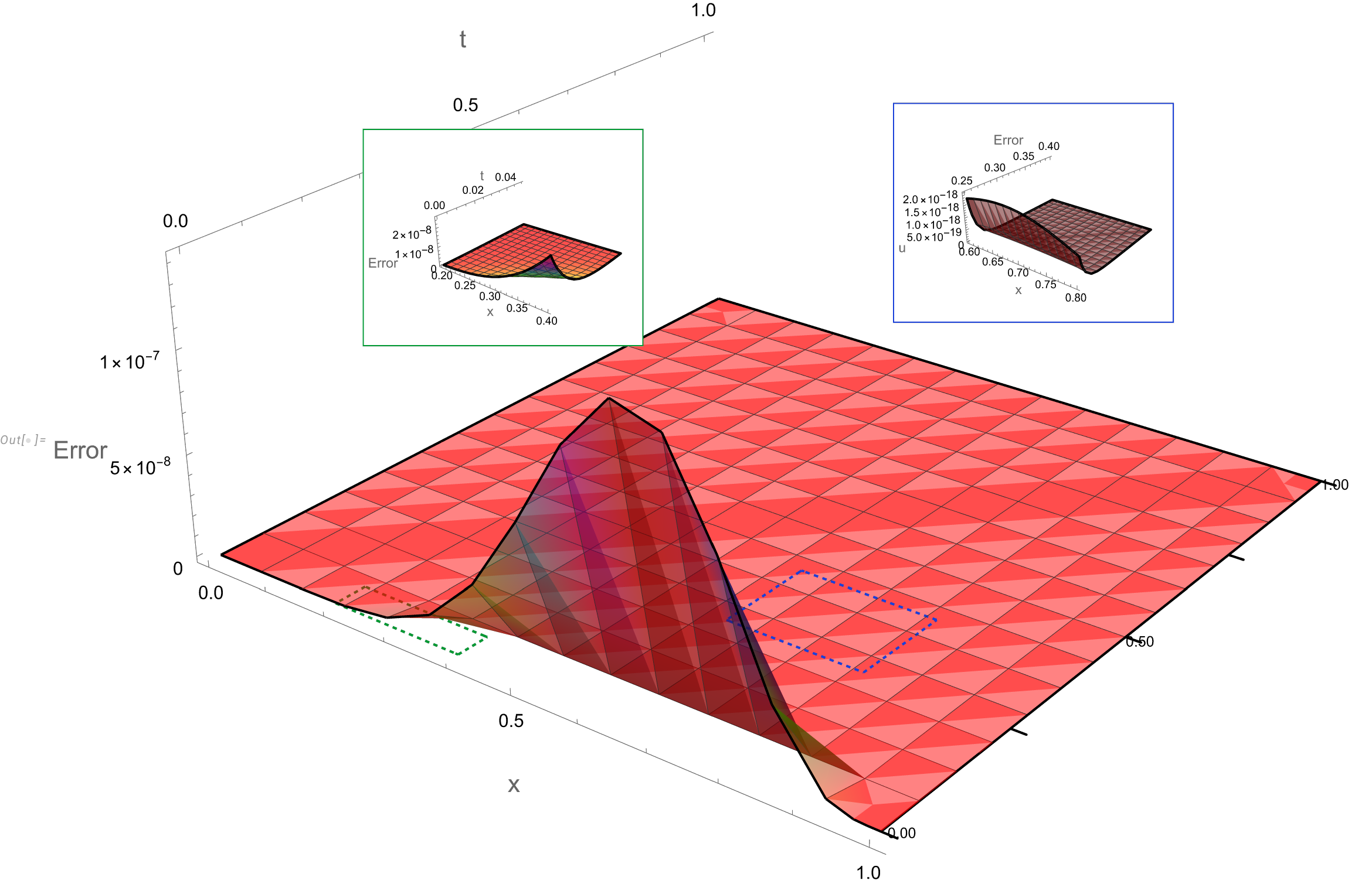
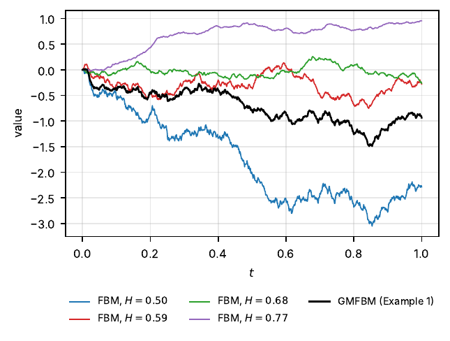
I also combine semismooth Newton methods with moving-least-squares collocation for pricing and sensitivity analysis under generalized mixed fractional Brownian motion, where memory effects make the paths neither Markovian nor semimartingale.
Nonlocal mechanics: fracture, fatigue & granular crushing
Concrete, rock, ceramics, glass, and the crushable grains of sand all fail the same way: cracks nucleate, grow, branch, and break the material into fragments. Standard tools are weakest here — cohesive-zone and continuum-damage models need crack paths specified in advance, and the discrete-element method treats grains as rigid bodies that cannot break. My work develops computational solid mechanics in which fracture, crushing, and fatigue emerge from the constitutive law itself, with the guarantees an engineer needs to rely on them.
The blended model for quasi-brittle fracture
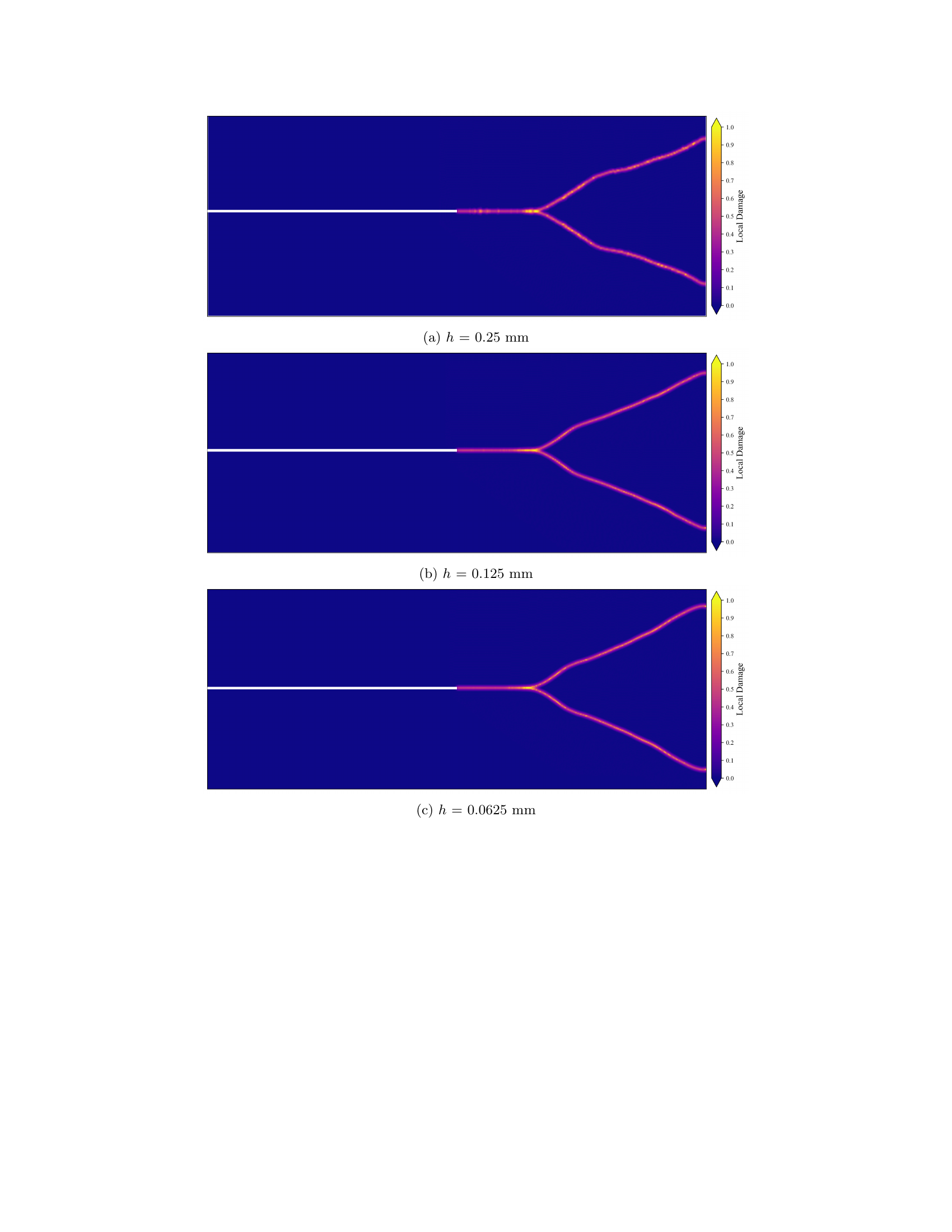
With S. Coskun and R. Lipton we introduced the blended model, which couples a nonlocal (peridynamic) force law with a two-point phase field that is an algebraic function of each bond’s strain history — so damage needs no extra diffusion equation and the displacement remains the only unknown. The displacement–damage pair is the unique solution of a single momentum balance (a Banach fixed point); energy balance with nonnegative dissipation follows from the equation of motion rather than being imposed; and for flat cracks the failure energy factors, through Crofton’s formula, into the Griffith energy \(\mathcal{G}_c\,\mathcal{H}^{d-1}\), independently of the horizon. With only three material constants beyond elasticity — all measurable in standard tests — the model reproduces cyclic load–CMOD curves of concrete beams, the structural size effect, mixed-mode crack paths, and dynamic crack branching in glass. (Coskun, Damircheli, Lipton, J. Mech. Phys. Solids, 2025)

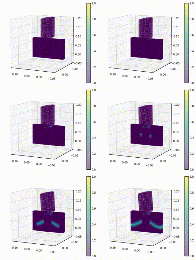
Ongoing work closes two physical gaps the validation exposed. A state-based blended model allows any Poisson ratio and introduces separate mode-I/mode-II damage channels plus damage–plasticity, so simulated unloading leaves residual strain as experiments do. A fatigue extension replaces the maximum-strain damage law with a bond-wise strain-path functional that accumulates damage above an endurance threshold, so \(S\)–\(N\) curves and Paris-type crack growth follow from the constitutive law rather than being fitted.
Crushing and comminution of 3D granular aggregates
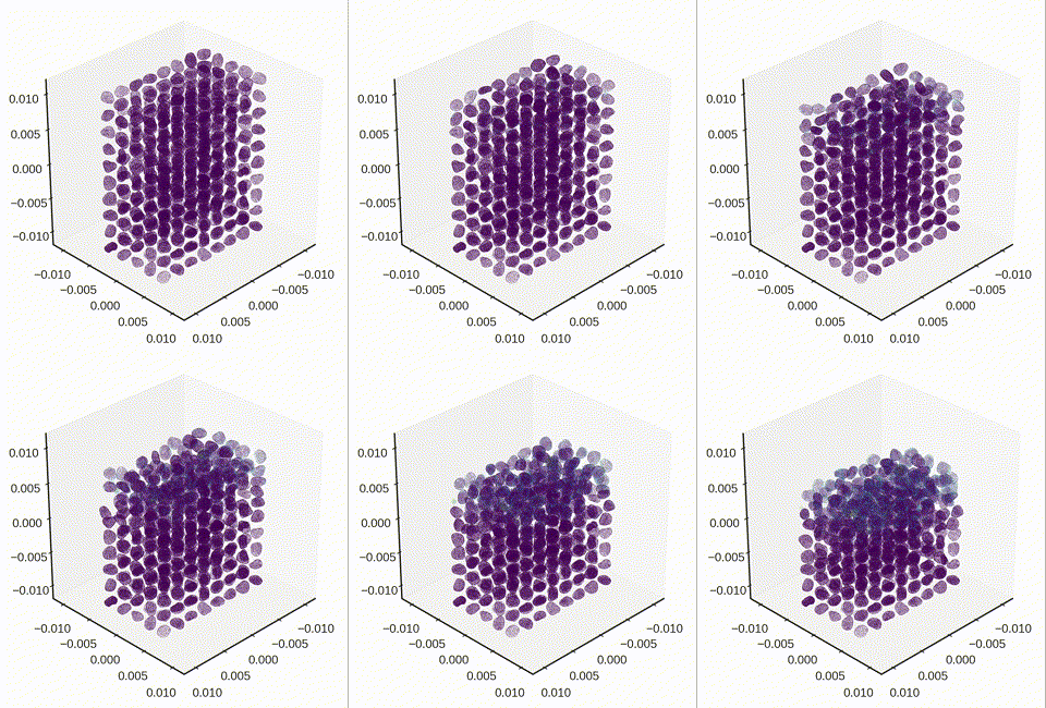
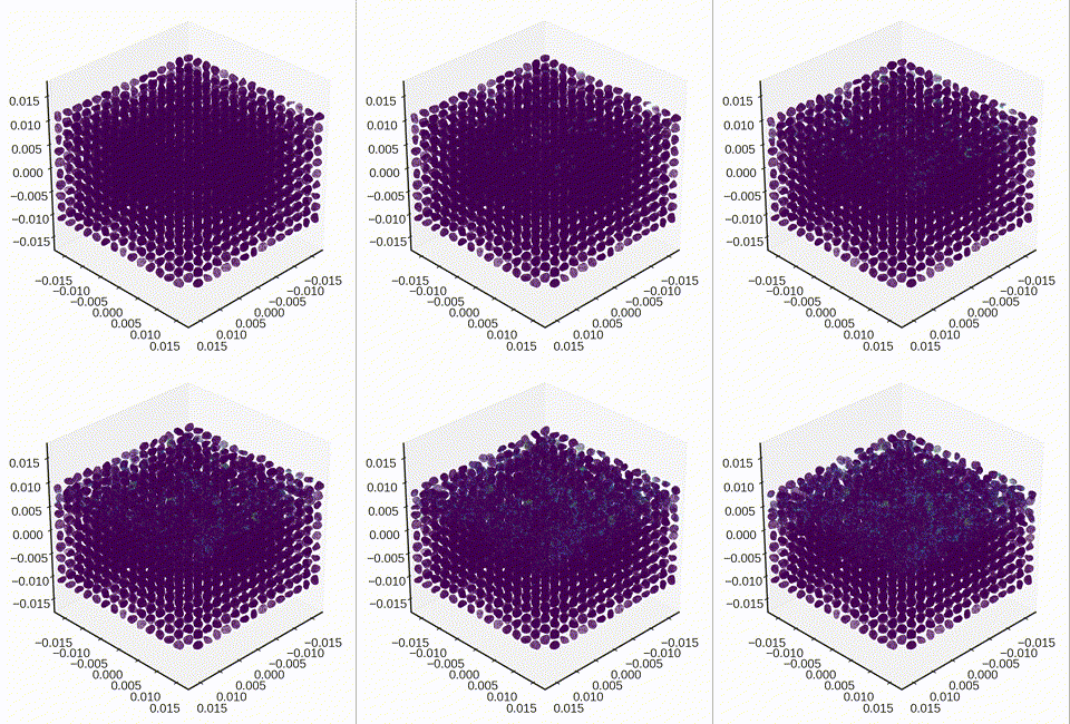
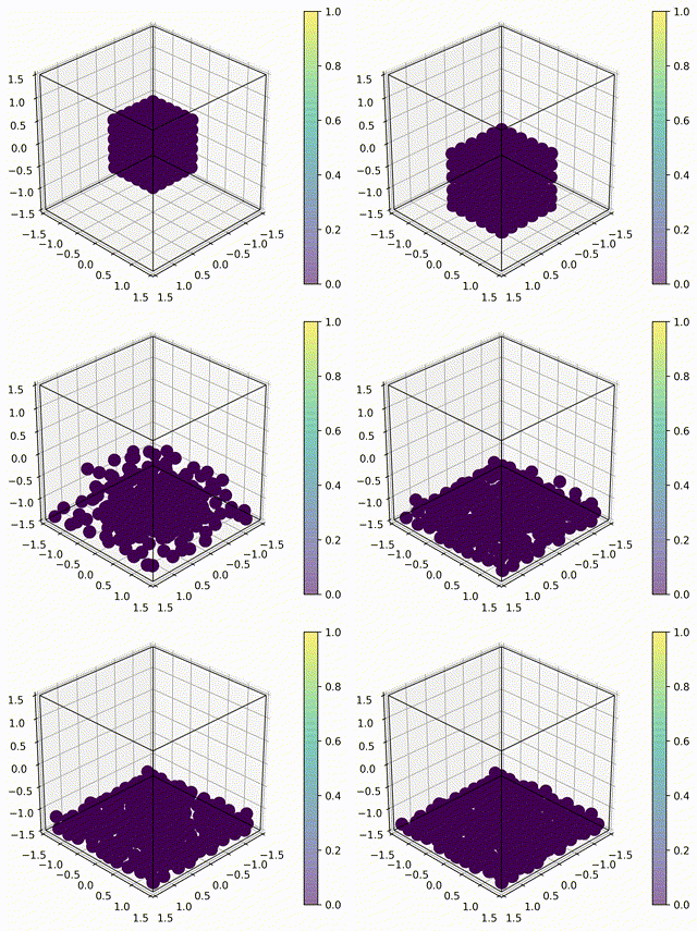
With D. Bhattacharya and R. Lipton I developed PeriGrain3D, a 3D framework in which every grain of an aggregate is a fracturing peridynamic body. Grains interact through nonlocal repulsion, regularized Coulomb friction, and contact damping; fragments of the same grain interact through self-contact once their bonds break; and rigid walls act through closed-form spherical-cap formulas, so no wall mesh is needed. Fracture is irreversible bond deletion and fragments are the connected components of the remaining bond graph, so crushing and comminution emerge from the dynamics with no crack tracking. The framework is verified against Hertz contact and the Kalthoff–Winkler experiment, and it quantifies how grain shape (solid, hollow, nonconvex) controls the strength of the aggregate. (Bhattacharya, Damircheli, Lipton — submitted, arXiv:2506.05362)

Within a compacted aggregate, individual grains pass from intact, through cracking, to full comminution:
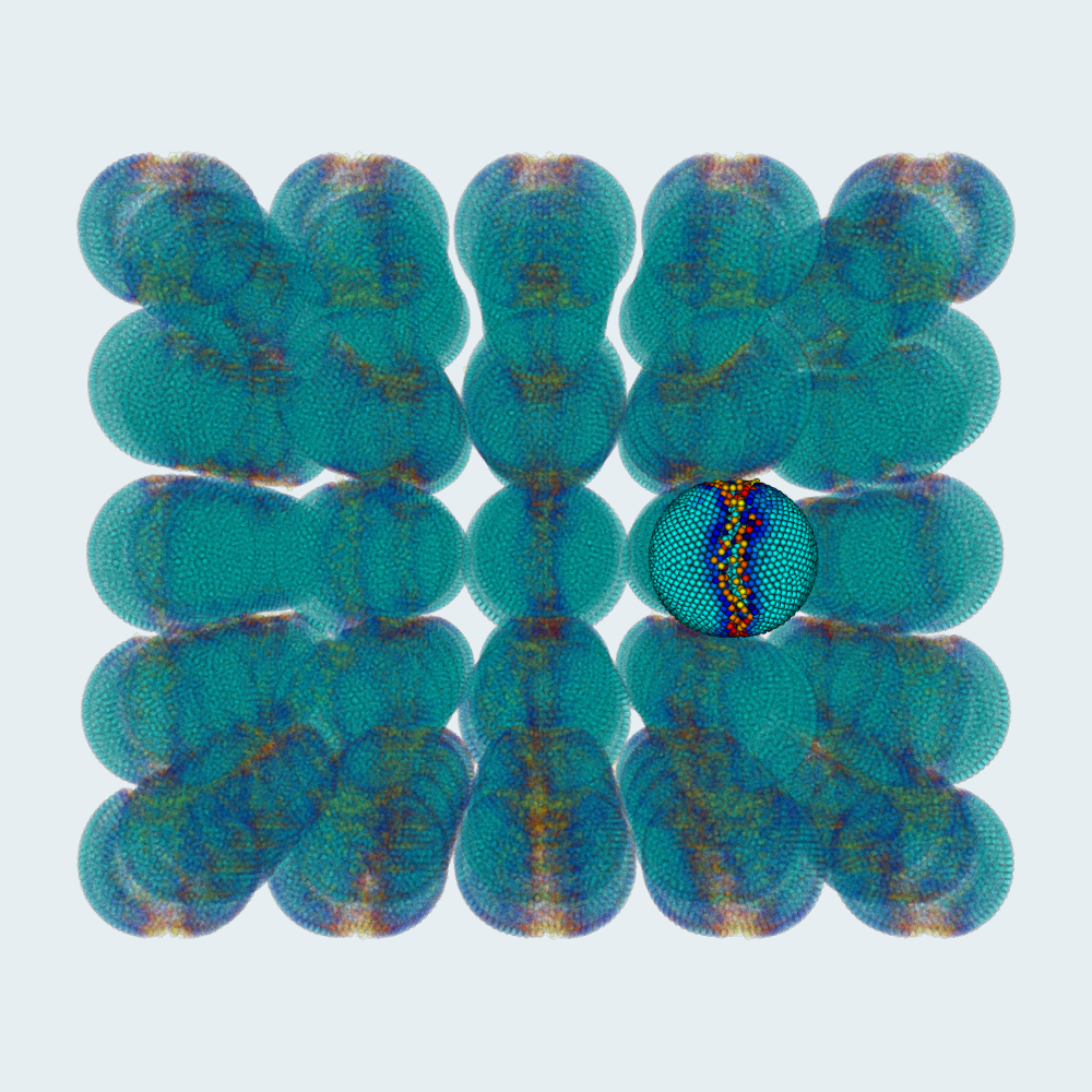
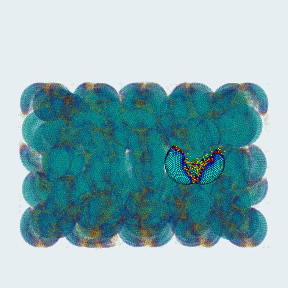
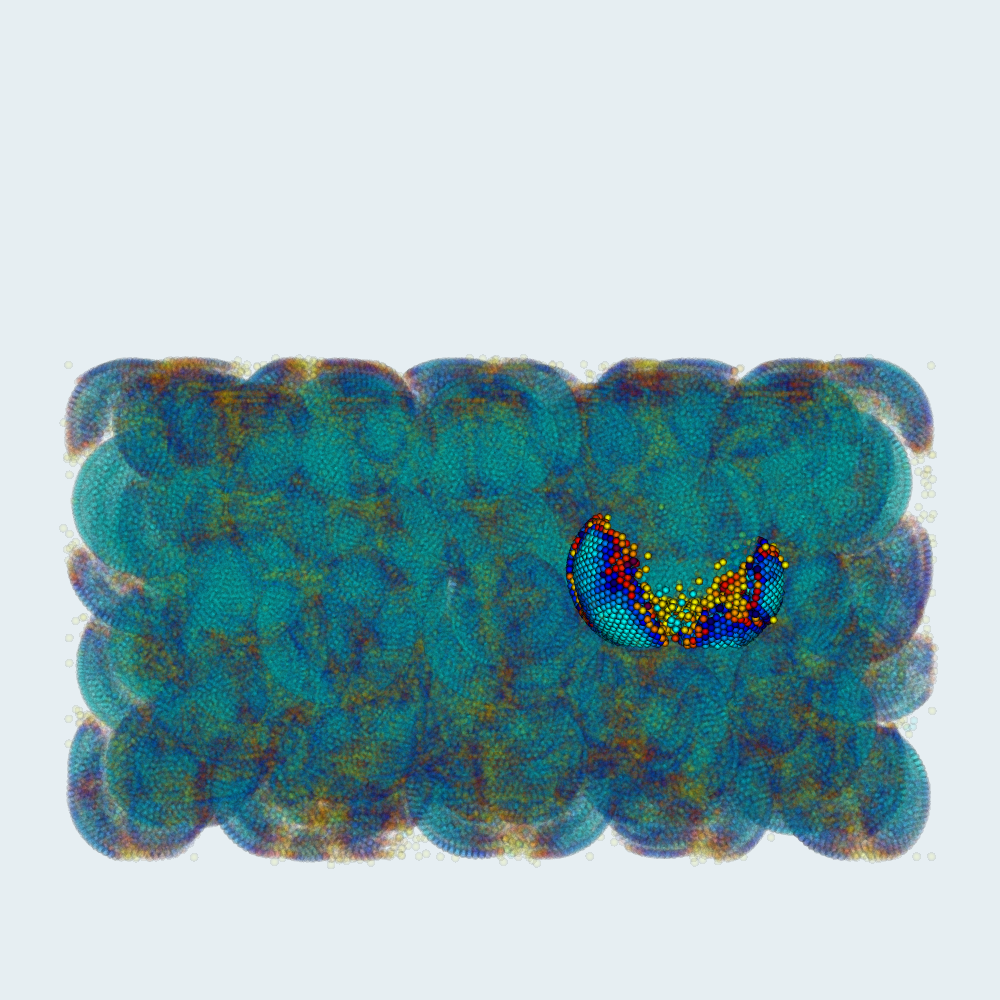
These simulations have been scaled to aggregates of up to 1,000 grains (X-ray-CT-reconstructed sand and hollow spheres, about 1.3 million material points) on up to 1,600 cores of LSU’s SuperMIC cluster. A companion study turns the simulator into a computational laboratory and defines an accuracy–cost map — the cheapest specimen size that meets a prescribed error tolerance for each quantity of interest — which matters when choosing a representative volume element for a multiscale model.
The simulation has a well-defined answer
Bond breaking makes the internal force a discontinuous function of the state, so a fracture code integrates a hybrid, event-driven dynamical system. For the semi-discrete scheme PeriGrain3D integrates, we proved existence of a unique global solution with irreversible bond breaking — each bond breaks at most once, and events cannot accumulate in finite time (no Zeno behavior) — and that hard damage is precisely what defeats the standard fixed-point argument in the continuum. A simulation can only be trusted once the program it implements has a well-defined answer.
Certified computation & scientific machine learning
Machine-learned models now price contracts, predict fracture, and stand in for expensive simulations inside design loops. They are fast, but they fail silently — giving no warning when a query leaves the training distribution, a constraint is violated, or training has converged to the wrong answer. My research asks: how can we certify, for a given input and at run time, that a computed or learned answer is correct?
Guaranteed error bounds for neural solutions of free-boundary problems
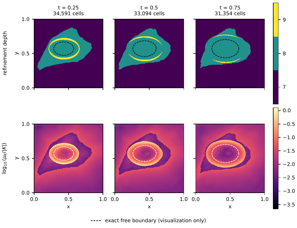
Constrained problems — obstacles, free boundaries, contact — are where neural PDE solvers fail most quietly, because a network can look accurate while violating the constraint. I proved and implemented guaranteed error bounds for neural approximations of parabolic obstacle problems (variational inequalities that include American option pricing and Stefan-type melting). The key idea is to certify not the network \(v\) but its feasible projection \(\hat v = \max\{v, g\}\), which removes every constraint-violation term and every hard-to-estimate stability constant from the bound. All integrals are evaluated with outward-rounded Taylor-model (interval) enclosures, so the certificate is a mathematical guarantee on any partition: adaptivity changes the cost, never the validity. Compared with the route through classical estimators, the constants are about \(59\times\) (1D) and \(237\times\) (2D) smaller. Just as important, the certificate explains failures — in an elliptical test case it localized the error to the free boundary and revealed that penalty-based training had collapsed the learned Lagrange multiplier to zero. (preprint, arXiv:2610.24202)
Run-time accept/reject certificates for surrogates
I also build query-wise certificates for reduced-order (POD) and neural operator (DeepONet, POD-NN) surrogates of the nonlocal CGMY pricing model. The certificate is a computable two-sided bound on the residual in the correct dual norm, followed by an accept / correct / fall-back-to-solver rule. Two ideas make it cheap: a closed-form, parameter-explicit lower bound on the operator spectrum (replacing numerical eigenvalue audits), and empirical interpolation applied to the one-variable Fourier symbol instead of to matrices, which gives a certificate whose online cost is independent of the mesh (milliseconds). In all tests the certificate never accepted an inaccurate answer, and it separated good from bad out-of-distribution predictions far more reliably than a “reject outside the training box” rule — while honestly reporting the negative result that in low dimension the tested neural surrogates offered no speed advantage over a well-structured solver.
I am also combining topological data analysis, graph neural networks, and classical domain decomposition into neural domain decomposition with convergence guarantees: the Mapper algorithm proposes overlapping subdomains, local learned corrections are coupled by an additive Schwarz iteration, and we prove an inexact-convergence theorem in which the global error contracts at a rate set by the cover plus a floor proportional to the local residual.
Earlier foundations
Variational inequalities and sensitivity analysis
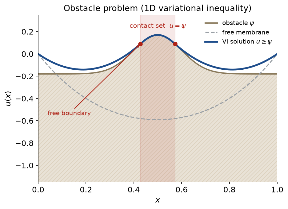
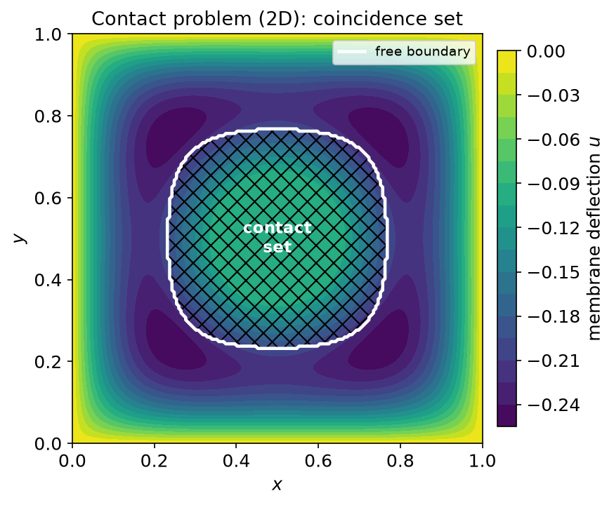
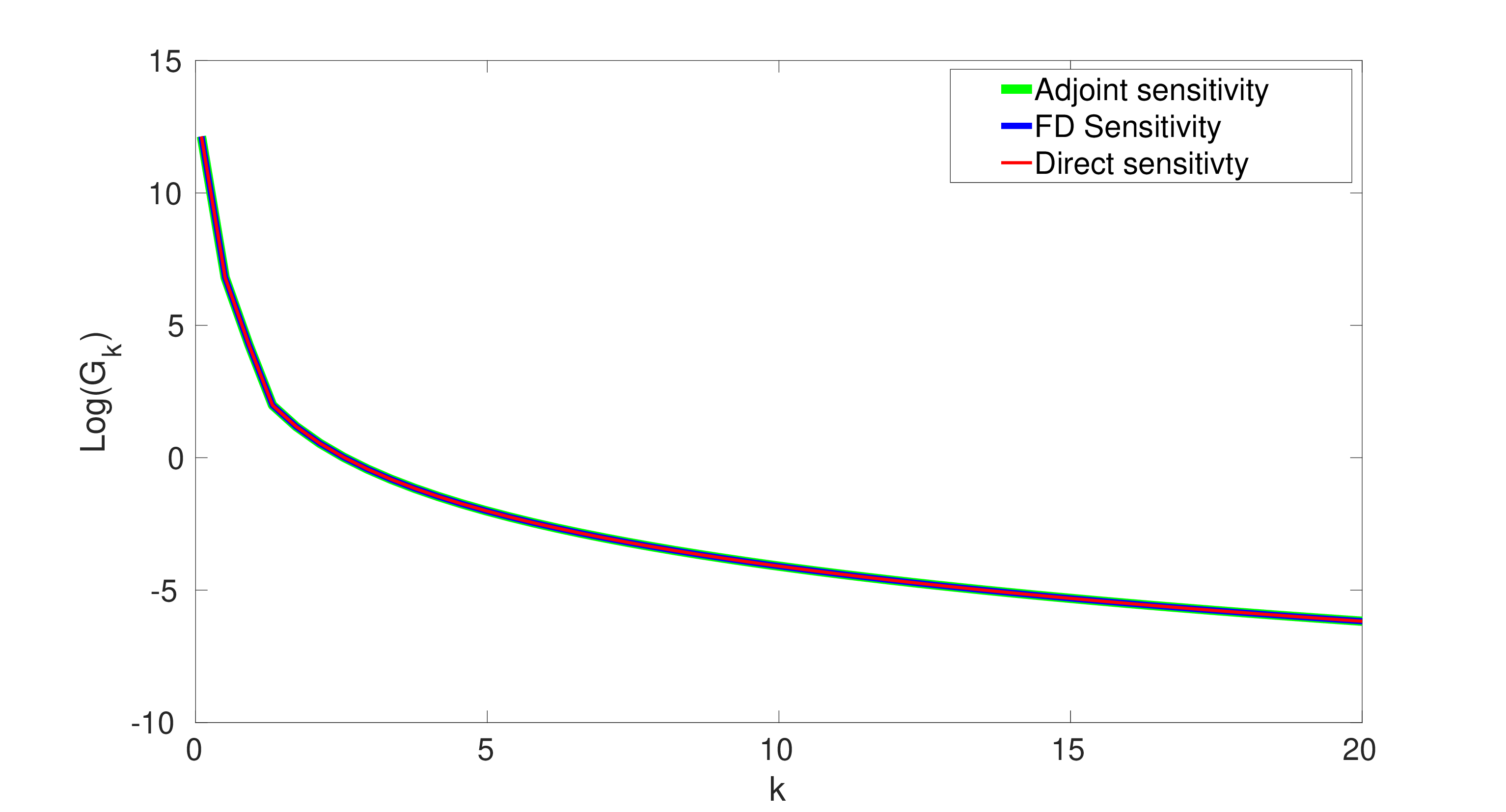
My engineering doctorate developed stable solution approaches with semismooth Newton methods and sensitivity analysis for variational inequalities arising in contact, plasticity, and phase change, with applications to design optimization. Contact, plasticity, and phase change (melting) share one mathematical form: a variational inequality in which the solution is constrained and a free boundary separates the active (contact) region from the free region — the quantity of greatest interest and the hardest to resolve. (Damircheli, Bhatia, AIAA SciTech, 2019)
Stochastic boundary value problems
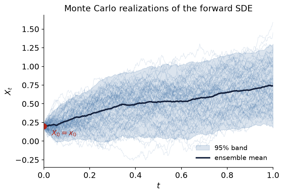
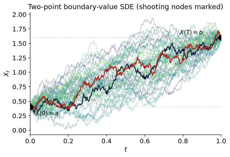
My master’s research concerned the numerical solution of stochastic differential equations with multi-point boundary conditions, whose solutions anticipate the noise. With A. Foroush Bastani I developed an adaptive multiple-shooting method that places shooting points along each sample path, and proved that it inherits the strong order of the underlying stochastic Runge–Kutta integrator. These SDEs arise in smoothing and maximum-a-posteriori estimation of diffusion trajectories, wave motion in random media, stochastic optimal control, and reciprocal processes, and from Rothe’s-method semi-discretization of stochastic PDEs. (Foroush Bastani, Damircheli, Numer. Algorithms, 2017)